
TaylorDiagram#
This notebook is a simple example of the GeoCAT-viz class TaylorDiagram class.
# Import packages:

import matplotlib.pyplot as plt
import numpy as np

import geocat.viz as gv
# Create sample data:
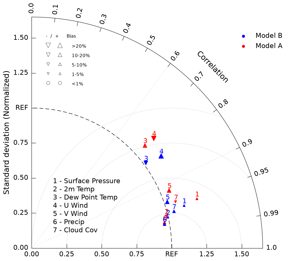
# Model A
a_sdev = [1.230, 0.988, 1.092, 1.172, 1.064, 0.966, 1.079] # normalized standard deviation
a_ccorr = [0.958, 0.973, 0.740, 0.743, 0.922, 0.982, 0.952] # correlation coefficient
a_bias = [2.7, -1.5, 17.31, -20.11, 12.5, 8.341, -4.7] # bias (%)
# Model B
b_sdev = [1.129, 0.996, 1.016, 1.134, 1.023, 0.962, 1.048] # normalized standard deviation
b_ccorr = [0.963, 0.975, 0.801, 0.814, 0.946, 0.984, 0.968] # correlation coefficient
b_bias = [1.7, 2.5, -17.31, 20.11, 19.5, 7.341, 9.2]
# Sample Variable List
var_list = ['Surface Pressure', '2m Temp', 'Dew Point Temp', 'U Wind', 'V Wind', 'Precip', 'Cloud Cov']
# Create figure and TaylorDiagram instance
fig = plt.figure(figsize=(10, 10))
taylor = gv.TaylorDiagram(fig=fig, label='REF')

# Draw diagonal dashed lines from origin to correlation values
# Also enforces proper X-Y ratio
taylor.add_corr_grid(np.array([0.6, 0.9]))

# Add models to Taylor diagram
taylor.add_model_set(a_sdev,
                  a_ccorr,
                  percent_bias_on=True, # indicate marker and size to be plotted based on bias_array
                  bias_array=a_bias, # specify bias array
                  color='red',
                  label='Model A',
                  fontsize=16)

taylor.add_model_set(b_sdev,
                  b_ccorr,
                  percent_bias_on=True,
                  bias_array=b_bias,
                  color='blue',
                  label='Model B',
                  fontsize=16)

# Add model name
taylor.add_model_name(var_list, fontsize=16)

# Add figure legend
taylor.add_legend(fontsize=16)

# Add bias legend
taylor.add_bias_legend()

# Add constant centered RMS difference contours.
taylor.add_contours(levels=np.arange(0, 1.1, 0.25),
                 colors='lightgrey',
                 linewidths=0.5);